Section 3.3 Investigation 1.9: Kissing the Right Way (cont.)
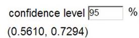
Recall the study published in Nature that found 64.5% of 124 kissing couples leaned right to kiss (Investigation 1.6). We previously used simulation and the binomial distribution to determine which values were plausible for the underlying probability that a kissing couple leans right (\(\pi\)). In particular, we found 0.5 and 0.74 were not plausible values for \(\pi\) but 0.6667 was. The 95% Clopper-Pearson Binomial confidence interval was (0.554, 0.729). Now you will consider applying the normal model as another method for producing confidence intervals for this parameter.
Checkpoint 3.3.1. Check CLT Validity Condition.
When you do not have a particular value to be tested for the process probability, it’s reasonable to use the sample proportion in checking the sample size condition for the CLT. (This is equivalent to making sure there are at least 10 successes and at least 10 failures in the sample.)
Checkpoint 3.3.2. Describe Distribution of Sample Proportion.
Hint.
Checkpoint 3.3.3. Estimate Standard Deviation.
Definition.
The standard error of the sample proportion, \(\text{SE}(\hat{p})\text{,}\) is an estimate for the standard deviation of \(\hat{p}\) (i.e., \(\text{SD}(\hat{p})\)) based on the sample data, found by substituting the sample proportion for \(\pi\text{:}\)
\begin{equation*}
\text{SE}(\hat{p}) = \sqrt{\frac{\hat{p}(1-\hat{p})}{n}}
\end{equation*}
Checkpoint 3.3.4. Find Largest Plausible Distance.
Now consider calculating a 95% confidence interval for the process probability \(\pi\) based on the observed sample proportion \(\hat{p}\text{.}\) What’s the largest distance you expect to see a sample proportion \(\hat{p}\) fall away from the underlying process probability \(\pi\text{?}\) [Hint: Assuming a normal distribution … 95% …]
Largest plausible distance =
Hint.
Checkpoint 3.3.5. Calculate Confidence Interval.
An approximate 95% confidence interval for the process probability based on the normal distribution would be \(\hat{p} \pm 2\sqrt{\hat{p}(1-\hat{p})/n}\text{.}\) That is, this interval extends two standard deviations on each side of the sample proportion. We know that for the normal distribution roughly 95% of observations (here sample proportions) fall within 2 SDs of the mean (here the unknown process probability), so this method will "capture" the process probability for roughly 95% of samples.
However, we should admit that the multiplier of 2 is a bit of a simplification. So how do we find a more precise value of the multiplier to use, including for values other than 95%?
Definition.
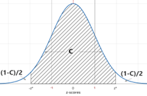
The \((100 \times C)\)% critical value, \(z^*\text{,}\) is the \(z\)-score value such that \(P(-z^* \leq Z \leq z^*) = C\) where \(C\) is any specified probability value, and \(Z\) represents a normal distribution with mean 0 and SD 1.
Note: We use the symbol \(z^*\) to distinguish this value, found based on the confidence level, from \(z_0\text{,}\) the observed \(z\)-score for the data.
Technology Detour — Finding Percentiles from the Standard Normal Distribution.
Use technology to more precisely determine the number of standard deviations that capture the middle 95% of the normal distribution with mean = 0 and standard deviation = 1. [Hint: In other words, how many standard deviations do you need to go on each side of zero to capture the middle 95% of the standard normal distribution?] Keep in mind that the \(z\)-value corresponding to probability \(C\) in the middle of the distribution, also corresponds to having probability \((1-C)/2\) in each tail.
Checkpoint 3.3.6. Finding Critical Values with Normal Probability Calculator.
In Normal Probability Calculator applet:
-
You can leave the mean set to zero and the standard deviation to 1 and the variable is "z-scores."
-
Check the box next to the first \(<\) sign and specify the probability value to correspond to the lower tail probability of interest: \((1-C)/2\text{.}\) Press Enter/Return and it will display the negative \(z^*\)-value.
Checkpoint 3.3.7. Finding Critical Values in R.
In R: The
iscaminvnorm function takes the following inputs:
-
Probability of interest (prob1)
-
mean = the mean of the normal distribution (default = 0)
-
sd = the standard deviation of the normal distribution (default = 1)
-
direction = whether the probability of interest was in the lower tail ("below") or the upper tail ("above"), in both tails ("outside"), or in the middle of the distribution ("between")
For example:
iscaminvnorm(prob1 = 0.95, direction = "between")
Checkpoint 3.3.8. Finding Critical Values in JMP.
In JMP using the Distribution Calculator in the ISCAM Journal File:
-
From the Distribution pull-down menu, select Normal (at the top of the list)
-
Specify the values for the mean (0) and standard deviation (1)
-
Change the Type of Calculation to
Input probability and calculate quantiles -
Select
Central Probabilityand specify the confidence level (e.g., 0.95) -
Press Enter/Return.
Checkpoint 3.3.9. Compare 90% Critical Value.
Find the critical value for a 90% confidence interval. Is it larger or smaller than with 95% confidence? Why does this make sense?
- Smaller
- The same
- Larger
Hint.
One Sample \(z\)-Confidence Interval (Wald Interval) for \(\pi\).
When we have at least 10 successes and at least 10 failures in the sample, an approximate confidence interval for \(\pi\) is given by:
\begin{equation*}
\hat{p} \pm z^* \sqrt{\frac{\hat{p}(1-\hat{p})}{n}}
\end{equation*}
where \(z^*\) corresponds to the confidence level.
Checkpoint 3.3.10. Identify Midpoint and Width.
Based on this formula, what (expression) is midpoint of the confidence interval? What (expression) is the width of the interval?
Hint.
Checkpoint 3.3.11. Effect of Confidence Level on Width.
How does increasing the confidence level affect the width of the interval?
- The width does not change
- Increases the width
- Decreases the width
Checkpoint 3.3.12. Effect of Sample Size on Width.
How does increasing the sample size affect the width of the interval?
- The width does not change
- Increases the width
- Decreases the width
Hint.
Definition.
The half-width of a confidence interval is also referred to as the margin of error.
So the above interval formula is of the common form: statistic \(\pm\) margin of error, where margin of error = critical value \(\times\) standard error of statistic. Here, margin of error = \(z^* \sqrt{\hat{p}(1-\hat{p})/n}\text{.}\)
Although 95% is the most common confidence level, a few other confidence levels and their corresponding critical values are shown in the table below.
| Confidence level | 90% | 95% | 99% | 99.9% |
|---|---|---|---|---|
| Critical value \(z^*\) | 1.645 | 1.960 | 2.576 | 3.291 |
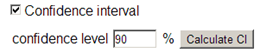
Checkpoint 3.3.14. Calculate and Compare 90% Interval.
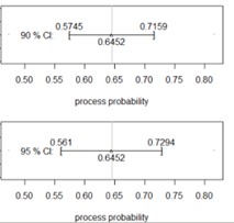
Use technology (see Technology Detour below) to find and report the 90% \(z\)-confidence interval for the probability that a kissing couple leans to the right. How do the midpoint and width of the 90% confidence interval compare to those of the 95% confidence interval?
90% interval:
Comparison:
Solution.
If the confidence level is 90%, then use \(z^* = 1.645\)
\(0.645 - 1.645 \times 0.043 = 0.5743\)
\(0.645 + 1.645 \times 0.043 = 0.7157\)
I am 90% confident that between 57.43% and 71.57% of kissing couples turn to the right.
Midpoint = \((0.5743 + 0.7157)/2 = 0.645\) (same as with the 95% confidence interval)
Width = \(0.7157 - 0.5743 = 0.142\) (smaller than for the 95% confidence interval)
\(2(1.645)(0.043) = 0.142\)
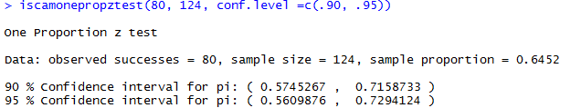
Technology Detour — One Proportion \(z\)-Confidence Intervals.
Checkpoint 3.3.15. \(z\)-interval with R.
Use
iscamonepropztest(observed, n, hypothesized, alternative="greater", "less," or "two.sided", conf.level)
You can enter either the number of successes or the proportion of successes (\(\hat{p}\)) for the "observed" value. If you don’t specify a hypothesized value and alternative, be sure to label the confidence level.
For example:
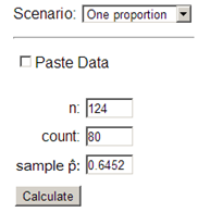
iscamonepropztest(observed=80, n=124, conf.level=0.95)
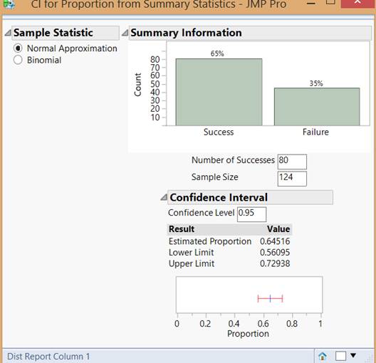
Checkpoint 3.3.16. \(z\)-interval with JMP.
-
Specify Raw Data (column of outcomes) or Summary Stats
-
With Summary Stats, keep the radio button set to
Normal Approximation
Checkpoint 3.3.17. \(z\)-interval with Theory-Based Inference applet.
Using the Theory-Based Inference applet:
-
Keep the pull-down menu set to
One proportion. -
Specify the sample size \(n\) and either the count or the sample proportion. Or check the
Paste Databox and paste in the individual outcomes (check theIncludes headerbox if you are also copying over the variable name). -
Press
Calculate. -
Check the box for
Confidence interval -
Change the confidence level from 95 to 90%
-
Press the
Calculate CIbutton
Checkpoint 3.3.18. Compare to Exact Binomial Intervals.
Hint.
Sample Size Determination.
Checkpoint 3.3.19. Determine Required Sample Size.
Suppose you are planning your own study about kissing couples. Before you collect the data, you know you would like the margin of error to be at most 3 percentage points and that you will use a 95% confidence level. Use this information to determine the sample size necessary for your study.
[This is a very common question asked of statisticians. Think about how to determine this using the \(z\)-interval formula. What information do you know? What information are you looking for?]
Approach 1: Use the sample proportion found in the original study as an estimate for the unknown value of \(\pi\text{.}\)
\(n =\)
Approach 2: Without a preliminary study, you can use 0.5 as an estimate of this probability.
\(n =\)
Hint.
Solution.
\(z^* \sqrt{\hat{p}(1-\hat{p})/n} = 0.03\)
Approach 1: Use the previous \(\hat{p} = 0.645\text{.}\)
Approach 2: Using 0.50
Checkpoint 3.3.20. Compare Sample Size Approaches.
We can solve for \(n\) by inverting the formula for the margin of error, assuming a value for \(\pi\text{.}\) The largest value for the margin of error occurs when \(\pi = 0.50\text{,}\) so that value can be used for a conservative estimate of the necessary sample size. You should always round your value up to the next integer to also ensure the margin of error won’t exceed the specification. Notice that this calculation is much more difficult with a binomial confidence interval which does not have a simple formula to manipulate.
Subsection 3.3.1 Practice Problem 1.9A
Recall from Practice Problem 1.8B that a student wanted to assess whether her dog Muffin tends to chase her blue ball and her red ball equally often when they are rolled at the same time. The student rolled both balls a total of 96 times, each time keeping track of which ball Muffin chased. The student found that Muffin chased the blue ball 52 times and the red ball 44 times. We arbitrarily decided to treat the blue ball as "success."
Checkpoint 3.3.21. Check Validity of \(z\)-procedures.
Is using theory-based \(z\)-procedures valid in this study? How are you deciding?
Checkpoint 3.3.22. Calculate 95% Confidence Interval.
Determine and interpret a 95% \(z\)-confidence interval.
Checkpoint 3.3.23. Compare Margins of Error.
Report the margin of error of your interval. Determine and compare to the margin of error change if with a 99% confidence level.
Checkpoint 3.3.24. Determine Required Sample Size.
What would be the necessary sample size if we wanted a margin of error of 0.01 for a confidence level of 95%? Explain how you are finding this.
Subsection 3.3.2 Practice Problem 1.9B
Checkpoint 3.3.25. Understanding Confidence Intervals.
In an actual study, how do you know whether your interval actually contains the value of the unknown parameter?
Solution.
In an actual study, you never know for certain whether your specific interval contains the unknown parameter. The parameter is a fixed value, and your interval either contains it or doesn’t. The confidence level refers to the long-run proportion of intervals that would contain the parameter if we repeated the study many times.
Checkpoint 3.3.26. Standard Deviation vs Standard Error.
What is the distinction between standard deviation and standard error?
Solution.
Standard deviation refers to the actual variability in the distribution (e.g., \(\text{SD}(\hat{p}) = \sqrt{\pi(1-\pi)/n}\)), which depends on the unknown parameter \(\pi\text{.}\) Standard error is an estimate of the standard deviation calculated from the sample data (e.g., \(\text{SE}(\hat{p}) = \sqrt{\hat{p}(1-\hat{p})/n}\)), where we substitute the sample proportion for the unknown parameter.
Reconsider Muffin from Subsection 3.2.2 and suppose our confidence interval is (0.2689, 0.4811). For each statement below, determine whether it is a valid or invalid interpretation of this confidence interval.
Checkpoint 3.3.27.
Statement 1: You are 95% confident that the interval (0.2689, 0.4811) contains the sample proportion of blue balls chased by Muffin.
- Valid
- Incorrect. We know the sample proportion exactly; there’s no need for a confidence interval for it. The confidence interval is for the parameter (the true probability), not the sample proportion.
- Invalid
- Correct! We know the sample proportion exactly; there’s no need for a confidence interval for it. The confidence interval is for the parameter (the true probability), not the sample proportion.
Checkpoint 3.3.28.
Statement 2: There is a 95% chance that the interval (0.2689, 0.4811) captures the probability Muffin chasing the blue ball.
- Valid
- Incorrect. This makes it sound like the parameter is random, when it’s actually fixed. The interval is what’s random. Once we’ve constructed this specific interval, it either contains the parameter or it doesn’t.
- Invalid
- Correct! This makes it sound like the parameter is random, when it’s actually fixed. The interval is what’s random. Once we’ve constructed this specific interval, it either contains the parameter or it doesn’t.
Checkpoint 3.3.29.
Statement 3: 95% of the time the interval (0.2689, 0.4811) contains the probability of Muffin chasing the blue ball.
- Valid
- Incorrect. This specific interval is fixed; it doesn’t change. The correct interpretation is about the procedure (95% of intervals constructed this way contain the parameter), not this specific interval.
- Invalid
- Correct! This specific interval is fixed; it doesn’t change. The correct interpretation is about the procedure (95% of intervals constructed this way contain the parameter), not this specific interval.
Checkpoint 3.3.30.
Statement 4: In the long run, 95% of sample proportions fall in between 0.2689 and 0.4811.
- Valid
- Incorrect. This confuses the confidence interval for the parameter with the distribution of sample proportions. The confidence interval tells us about plausible values for the parameter, not where sample proportions fall.
- Invalid
- Correct! This confuses the confidence interval for the parameter with the distribution of sample proportions. The confidence interval tells us about plausible values for the parameter, not where sample proportions fall.
Checkpoint 3.3.31.
Statement 5: If the null hypothesis is true, there is a 95% chance the interval contains the parameter.
- Valid
- Incorrect. Confidence intervals don’t depend on whether a null hypothesis is true or not. The confidence level comes from the sampling distribution, not from any hypothesis.
- Invalid
- Correct! Confidence intervals don’t depend on whether a null hypothesis is true or not. The confidence level comes from the sampling distribution, not from any hypothesis.
Checkpoint 3.3.32.
Statement 6: I am 95% confident that Muffin chases the blue ball between 27% and 48% of the time.
- Valid
- Correct! This correctly expresses confidence about the parameter (the underlying probability/long-run proportion). This is a proper interpretation of a confidence interval.
- Invalid
- Incorrect. This is actually a valid interpretation because it correctly expresses confidence about the parameter (the underlying probability/long-run proportion).
You have attempted of activities on this page.
