Section 3.4 Investigation 1.10: Heart Transplant Mortality (cont.)
Recall Investigation 1.4, where you learned that 8 of the 10 most recent heart transplantation operations at St. George’s Hospital resulted in a death.
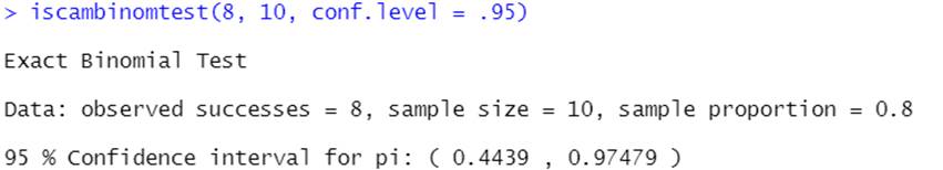
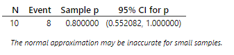
Use technology to find the "exact binomial" (Clopper-Pearson) 95% confidence interval for the probability of death in the heart transplantation process at St. George’s Hospital.
Checkpoint 3.4.1. Exact Binomial Technology - R.
Checkpoint 3.4.2. Exact Binomial Technology - JMP.
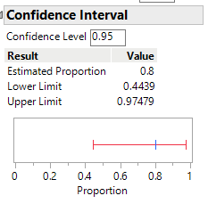
Checkpoint 3.4.3. Report Exact Binomial Interval.
Solution.
The midpoint of this interval is (.4439 + .9748)/2 = 0.709 which is lower than \(\hat{p}\) = 0.80. This makes sense as if we observed \(\hat{p}\) = 0.80, the largest \(\pi\) could be is 1.0 (.20 away) but \(\pi\) could conceivably be as small as 0.0 (.80 away), so we don’t want an interval that is symmetric around 0.80. The width is .9748 - .4439 = 0.531.
Checkpoint 3.4.4. Calculate 95% z-Confidence Interval.
Hint.
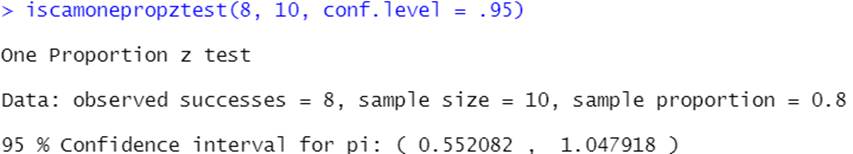
Use technology to verify your calculation of the one proportion \(z\)-interval (also called the Wald interval)
Checkpoint 3.4.5. Verify z-Interval with Technology - R.
Checkpoint 3.4.6. Verify z-Interval with Technology - JMP.
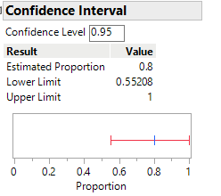
Checkpoint 3.4.7. Report z-Interval Results.
Checkpoint 3.4.8. Assess Validity of z-Interval.
Key Idea.
The confidence level of an interval procedure is supposed to indicate the long-run percentage of intervals that capture the actual parameter value, if repeated random samples were taken from the identical process. As such, the confidence level presents a measure of the reliability of the method. A confidence interval procedure is considered valid when the achieved long-run coverage rate matches (or comes close to) the stated (aka nominal) confidence level.
Statistical confidence is a statement about the method, not a probability statement about an individual interval.
To consider whether the one sample \(z\)-interval is valid for this study, we can pretend we know the process probability, generate many random samples from that process, calculate confidence intervals from the simulated samples, and see what percentage of these confidence intervals capture the actual value of the process probability that we specified.
Checkpoint 3.4.9. Explore Simulating Confidence Intervals Applet.
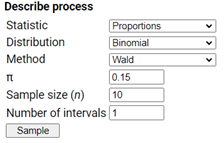
Open the Simulating Confidence Intervals applet.
Suppose the actual process probability of death is 0.15 and you plan to take a sample of 10 operations and apply the \(z\)-interval (aka Wald) method.
-
Set the value of \(\pi\) to 0.15 and the Sample size (n) to 10.
-
Press Sample.
-
Click on the interval to see the endpoint(s), midpoint, and width (verify).
Did you obtain the same interval as in (c)? Why or why not?
Did the interval succeed in capturing the value of \(\pi\text{,}\) which we set to be 0.15? How can you tell?
Checkpoint 3.4.10. Evaluate z-Interval Coverage Rate.
Change the Number of intervals to 100 and press Sample until you have at least 1,000 intervals in the Running total. How many of these random intervals succeed in capturing the actual value of the process probability (0.15)? Does this method appear to succeed in capturing the value of the parameter (which we assumed to be equal to 0.15) 95% "of the time"?
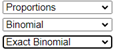
Because the \(z\)-interval procedure has the sample size conditions of the Central Limit Theorem, there are scenarios where we should not use this \(z\)-procedure to determine the confidence interval. In these cases, one option is to use the Exact Binomial distribution (Clopper-Pearson) method.
Checkpoint 3.4.11. Evaluate Exact Binomial Coverage Rate.

Checkpoint 3.4.12. Average Width of Exact Binomial Intervals.
The Clopper-Pearson method will have a coverage rate of at least 95%, but tends to be "conservative," meaning the coverage rate is higher than 95% so the intervals are longer than they need to be. The method is also fairly complicated (as opposed to: "go two standard deviations on each side"). An alternative method that has been receiving much attention of late is often called the Plus Four procedure:
Definition: Plus Four 95% Confidence Interval for \(\pi\).
-
Increase the number of successes by two and the sample size by four, and calculate a new proportion: \(\tilde{p} = (X + 2)/(n + 4)\text{.}\) Make this value the midpoint of the interval.
-
Use the \(z\)-interval procedure as above for the augmented sample size of \((n + 4)\text{:}\) \(\tilde{p} \pm z^* \sqrt{\frac{\tilde{p}(1-\tilde{p})}{n+4}}\)
In short, with 95% confidence, the idea is to pretend you have 2 more successes and 2 more failures than you really did. For confidence levels other than 95%, researchers have recommended using the Adjusted Wald method: \(\tilde{p} = (X + 0.5(z^*)^2)/(n + (z^*)^2)\) and \(\tilde{n} = n + (z^*)^2\) so the interval becomes \(\tilde{p} \pm z^* \sqrt{\frac{\tilde{p}(1-\tilde{p})}{\tilde{n}}}\text{.}\)
Checkpoint 3.4.13. Evaluate Plus Four Coverage Rate.
Investigate the reliability of the Plus Four procedure using the applet:
-
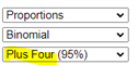
Use the Method pull-down menu to change from Exact Binomial to Plus Four (95%).
-
Generate at least 1,000 confidence intervals from a process with \(\pi = 0.15\) and \(n = 10\text{.}\)
Is this coverage rate close to 95%? Is this an improvement over the (Wald) \(z\)-interval?

Checkpoint 3.4.14. Average Width of Plus Four Intervals.
Checkpoint 3.4.15. Compare Plus Four to Exact Binomial Width.
Do these intervals tend to be narrower than intervals calculated using the Exact Binomial interval procedure?
- Yes
- No
Checkpoint 3.4.16. Compare Interval Midpoints.
Use the Method pull-down menu to toggle between the Wald and Plus Four intervals. [Hint: You can Sort the intervals first.] What do you notice about how the midpoints of the intervals compare? (Also think how \(\tilde{p}\) and \(\hat{p}\) differ, these are the values shown in the "Sample statistics (CI Midpoints)" graph.) Why is the change in the midpoints of the intervals useful in this scenario?
Checkpoint 3.4.17. Evaluate Blaker Method.
In the applet, change the number of intervals to 100. Press Reset. Use the pull-down menu to select the Blaker method (the Exact Binomial using the tail probabilities), and wait a bit. (If it’s just 100 at a time, it’s not too bad to hit Sample a few more times.) Report the percentage of intervals that capture the parameter AND the average width of these 100 intervals.
Running Total:
Average width:
Checkpoint 3.4.18. Assess Blaker Method.
Does this appear to be a 95% confidence interval procedure?
- Yes
- Correct! Especially if you look at a few hundred, about 95% of the intervals appear to capture the parameter.
- No
- Not quite. Look at the running total - it should be very close to 95%.
Checkpoint 3.4.19. Shortest Intervals.
In your simulations, which method(s) appear to have the shortest intervals?
- Binomial
- Not quite. The binomial intervals tend to be wider on average.
- Plus Four
- Correct! The Plus Four and Blaker methods tend to have shorter intervals than the binomial method.
- Blaker
- Correct! The Plus Four and Blaker methods tend to have shorter intervals than the binomial method.
Key Idea.
The Plus Four method is more likely to be a 95% confidence interval method than the one-sample \(z\)-interval method. It is never a bad idea to use the Plus Four method.
"Fudging our data" may seem like cheating, but there is actually some nice theory behind this method. The plus four adjustment is not that different in principle from the continuity correction we suggested with p-values. Many statisticians now recommend using this procedure over the one proportion \(z\)-interval procedure because it achieves the stated confidence level for any sample size and over the Clopper-Pearson binomial interval procedure because the intervals tend to be shorter (narrower). In fact, the more general case (something other than 95%) is becoming the default in many software packages. (The Blaker method in others.)
Checkpoint 3.4.20. Plus Four Interval for St. George’s Hospital.
Determine and then interpret a Plus Four confidence interval for the probability of a death during a heart transplant operation at St. George’s hospital. [Hints: You can do the calculation either by hand, first finding \(\tilde{p}\) and \(z^*\text{,}\) or with software (e.g., the Theory-Based Inference applet) by telling the technology there were 4 more operations consisting of two more deaths than in the actual sample. Note: You can’t use the Simulating Confidence Intervals applet to answer this question.]
Plus Four interval: (, )
Interpretation:
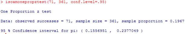
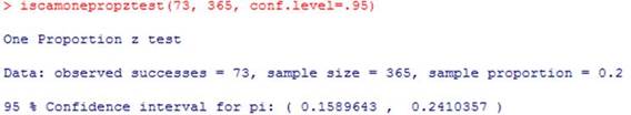
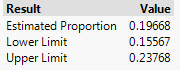
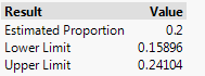
Checkpoint 3.4.21. Compare Intervals for Larger Study.
Subsection 3.4.1 Practice Problem 1.10A
Return to your exploration using the Simulating Confidence Intervals applet. Assume that \(\pi = 0.667\) is the probability that a kissing couple leans to the right.
Checkpoint 3.4.22. Evaluate Score Interval Method.
From the Method pull-down menu select the Score interval method. Evaluate the performance of this interval method, clearly explaining your steps. [Hint: Does the performance depend on the value of \(n\) that you use? What if you change the value of \(\pi\) to something closer to 0 or 1? Average widths?]
Solution.
The Score interval method performs well across different sample sizes and parameter values. The coverage rate is close to the nominal 95% confidence level even for small sample sizes and extreme values of \(\pi\text{.}\) As sample size increases, the average width of the intervals decreases while maintaining the appropriate coverage rate.
Checkpoint 3.4.23. Derive Score Interval Formula.
Starting with \(z = \frac{\hat{p} - \pi}{\sqrt{\pi(1-\pi)/n}}\text{,}\) use the quadratic formula to solve for \(\pi\) and verify the first formula for the Score interval.
Solution.
Starting with \(z = \frac{\hat{p} - \pi}{\sqrt{\pi(1-\pi)/n}}\text{,}\) square both sides and rearrange to get a quadratic equation in \(\pi\text{.}\) Using the quadratic formula yields the Score interval formula:
\(\frac{\hat{p} + \frac{z^2}{2n} \pm z\sqrt{\frac{\hat{p}(1-\hat{p})}{n} + \frac{z^2}{4n^2}}}{1 + \frac{z^2}{n}}\)
Checkpoint 3.4.24. Compare Score and Adjusted Wald Midpoints.
Show that the midpoint of the Score formula found in (b) simplifies to the midpoint of the Adjusted Wald procedure.
Solution.
The midpoint of the Score interval is \(\frac{\hat{p} + \frac{z^2}{2n}}{1 + \frac{z^2}{n}}\text{.}\) With \(z^* = 1.96 \approx 2\text{,}\) this becomes approximately \(\frac{\hat{p} + \frac{4}{2n}}{1 + \frac{4}{n}} = \frac{\hat{p} + \frac{2}{n}}{1 + \frac{4}{n}}\text{,}\) which matches the midpoint of the Adjusted Wald (Plus Four) procedure.
Checkpoint 3.4.25. Relate Adjusted Wald to Plus Four.
Show that with 95% confidence the midpoint of the Adjusted Wald procedure can be approximated with \(\frac{X + 2}{n + 4}\text{,}\) the Plus Four method.
Solution.
With \(z^* = 1.96 \approx 2\) for 95% confidence, the Adjusted Wald midpoint \(\frac{\hat{p} + \frac{z^{*2}}{2n}}{1 + \frac{z^{*2}}{n}}\) becomes \(\frac{\hat{p} + \frac{4}{2n}}{1 + \frac{4}{n}} = \frac{\hat{p} + \frac{2}{n}}{1 + \frac{4}{n}}\text{.}\) Since \(\hat{p} = \frac{X}{n}\text{,}\) this equals \(\frac{\frac{X}{n} + \frac{2}{n}}{1 + \frac{4}{n}} = \frac{\frac{X+2}{n}}{\frac{n+4}{n}} = \frac{X+2}{n+4}\text{,}\) which is the Plus Four method.
Subsection 3.4.2 Practice Problem 1.10B
Checkpoint 3.4.26. Probability of Selecting Capturing Interval.
Solution.
The probability is approximately 0.95 (or 95%). Since these are 95% confidence intervals, in the long run about 95% of the intervals will capture the true parameter value \(\pi\text{.}\) Therefore, randomly selecting one interval gives you about a 95% chance of selecting one that captures \(\pi\text{.}\)
Checkpoint 3.4.27. Probability for Specific Interval.
Solution.
The probability is either 0 or 1 - we just don’t know which! Once a specific interval is constructed, the parameter \(\pi\) either is or isn’t in that interval. The "95% confidence" refers to the method, not to any particular interval. If we were to use this method repeatedly, about 95% of the intervals constructed would contain \(\pi\text{.}\)
Checkpoint 3.4.28. Effect of Confidence Level.
In general, how does increasing the confidence level impact the width and coverage rate of a confidence interval procedure?
- Width decreases, coverage rate decreases
- Incorrect. To be more confident, we need a wider interval and higher coverage rate.
- Width decreases, coverage rate increases
- Incorrect. Higher confidence level requires a wider interval.
- Width increases, coverage rate increases
- Correct! Increasing confidence level requires a larger critical value, which increases the margin of error and makes the interval wider. It also increases the coverage rate - a higher percentage of intervals will capture the true parameter.
- Width increases, coverage rate decreases
- Incorrect. Higher confidence level means we capture the parameter more often, not less.
Checkpoint 3.4.29. Effect of Sample Size.
In general, how does increasing the sample size impact the width and coverage rate of a confidence interval procedure?
- Width decreases, coverage rate stays the same
- Correct! Larger sample sizes reduce the standard error, which decreases the margin of error and makes intervals narrower. For a valid confidence interval procedure, the coverage rate should remain at the stated confidence level (e.g., 95%) regardless of sample size.
- Width decreases, coverage rate increases
- Incorrect. While larger samples produce narrower intervals, the coverage rate should match the confidence level regardless of sample size for a valid procedure.
- Width stays the same, coverage rate stays the same
- Incorrect. Sample size affects the width through the standard error.
- Width increases, coverage rate stays the same
- Incorrect. Larger samples give more precise estimates with narrower intervals, not wider.
You have attempted of activities on this page.
